Graph Attention Networks
Graph Networks have been around for quite a while, and there are plenty of sources online that can give you a good overview.
This lesson from UvA Deep Learning Tutorials is a great start.
But often, the implementation gets quite a handful, and as a result, people skip. 😞
I tried to make a simple implementation, easy and intuitive.
Here we get the basic Graph Convolutional Layer, and the Graph Attention Layer, multi-headed! Hehe!
Graph Convolutional Layer
For a gentle start, let’s begin with a Graph Convolutional Network.
So suppose we have such a network where the adjacent nodes embeddings would be
- gathered,
- projected to another dimension
- and passed as an average.
That means, the embeddings are summed up, and then divided by the number of nodes where the embeddings are collected from.
Okay, a key point to note is that the neighbors of a node include itself too! The idea is to let a node embedding interact with neighbors and itself. So, 🙃.
As a result, the forward pass of the function would need the adjacency matrix, for gathering and averaging, along with the node features.
The resultant code looks like this :
class GCNLayer(nn.Module) :

    def __init__(self, d_in, d_out) :
        super().__init__()
        self.projection = nn.Linear(d_in, d_out)

    def forward(self, x, adj_hat) :
        # x : Node features : batch, n_nodes, d_in
        # adj_hat : adj matrix with self connections : batch, n_nodes, n_nodes

        x = self.projection(x) # to another dimension
        x = torch.bmm(adj_hat, x) # for all node embeddings, in a matrix form
        x = x / adj_hat.sum(dim = -1, keepdims = True) # averaging

        return x
And obviously, any kind of non-linearity is welcome.
This was rather simple, right? Well, the original paper does the averaging in a slightly different way.
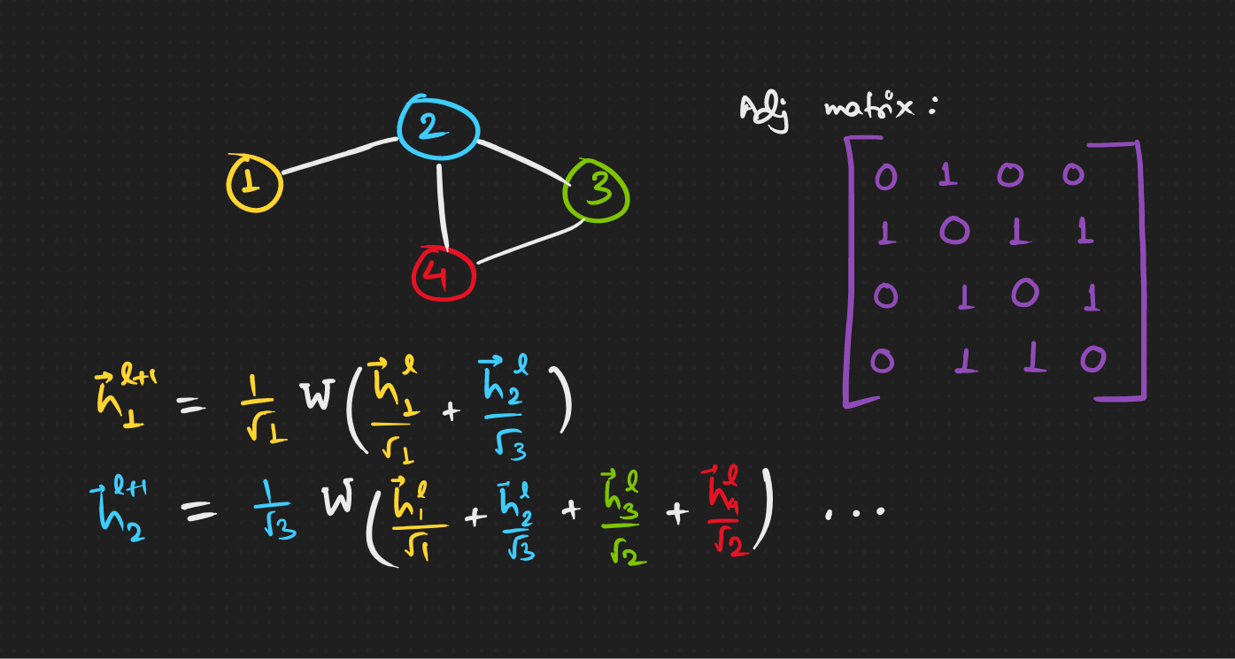
Originally each node embedding, while summing, has to be normalized by the square-root of the contributing node’s neighbourhood size and the square-root of the resulting node’s neighbourhood size.
Aaaah, let’s look at an example, with Adjacency matrix A as in the figure.

Hmm, can this be made into a matrix operation and get it done with at once?
Coside this matrix D, which is a diagonal matrix with elements equal to the number of neighbours of a node.
Being a diagonal matrix, inverting and raising it to some arbitrary power is easy. So now we have this,
And lastly, A with self connections would be \hat{A} ,
The following operation gives, (saving you some math, but feel free to do it on your own 😌)
which is the exact set of coefficients we need to calculate the next layer embeddings. 😇 Finally, we can reduce it to,
The code changes as :
class GCNLayerOrig(nn.Module) :

    def __init__(self, d_in, d_out) :
        super().__init__()
        self.projection = nn.Linear(d_in, d_out)

    def forward(self, x, adj_hat) :
        # x : Node features : batch, n_nodes, d_in
        # adj_hat : adj matrix with self connections : batch, n_nodes, n_nodes

        n_nodes = adj_hat.size()[1]
        adj = adj_hat - torch.eye(n_nodes) # without self connections

        d_hat = adj.sum(dim = -1)
        d_hat = torch.pow(d_hat, -0.5)
        d_hat = torch.diag_embed(d_hat) # batch, n_nodes, n_nodes

        dad = torch.bmm(torch.bmm(d_hat, adj_hat), d_hat) # normalizing matrix

        x = self.projection(x) # to another dimension
        x = torch.bmm(dad, x) # for all node embeddings, in a matrix form

        return x
And that’s the original GCN Layer. 😄
Graph Attention Layer + Multi Headed
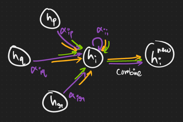
Much like how attention-networks provide us with a weighted average with the weights being dynamically computed, graph attention layer also does the same. Although it differs greatly in the way how these weights are calculated.
And we’ll get there soon, but let’s first see the modified equation for a layer’s node embeddings.
where
and a is another matrix for transforming the concatenated node embeddings to a scalar, ideally one scalar for each head.
Ahaha, point to note here is that, for N-headed attention, we’d need to split the embeddings to N parts.
Also, why the activation there? 🧐 My physics teacher, Praveen sir told me “to realize the importance of something, imagine what’d happen if it’s not there”.
So graphically, we’d have something like this…

Now, time to put it into some code. We’ll have a walkthrough and build it up. Okay? 🧐
I trust that skipping the initialization stuff won’t harm. So just going to the forward function. We have two inputs, x and adj_hat, with shapes (batch_size, n_nodes, d_in) and (batch_size, n_nodes, n_nodes) respectively.
x = self.projection(x) # transformed by W, has shape (B, N, heads x d_out)
x = x.view(B, N, self.n_heads, self.d_out) # x now has this shape
The most tricky part is to get the combinations of concatenated node embeddings efficiently. This is where most implementations would use some very complex black magic.
Let’s reverse engineer this. The last thing that gets multipled by a matrix for the attentions, has to have the shape (…, n_heads, 2 * d_out). Right?
And how many such combinations are there? That’s what we started with, we need all concatenations of two node embeddings. So, n_nodes x n_nodes. So the shape boils down to (batch_size, n_nodes x n_nodes, n_heads, 2 * d_out). 🤯
Now to get these complex looking repersentations. Hmm… 😮💨
Torch has blessed us with two functions.
🤌
repeat_interleave(repeats, dim)
This function would repeat a tensor, along dimension dim for repeats times, in a not so straight-forward manner. Maybe this will help. Say there’s a tensor of the form [[x1, x2], [x3, x4]] where all x have some n-dimensional shape.
repeat_interleave(2, dim = 1) would give [[x1, x1, x2, x2], [x3, x3, x4, x4]]
repeat((tuple with number of repeats each dimension))
Better to just go with the example, with the same previous x, repeat((1, 2, …)) would give [[x1, x2, x1, x2], [x3, x4, x3, x4]]
Now concatenating the two outputs along the last dimension does it. We would get the shape of x changed to (2, 2 x 2, 2 x n_dimensional). We use this for our case as follows.
# p.shape : B, N x N, n_heads, 2 x d_out
p1 = x.repeat_interleave(N, dim = 1)
p2 = x.repeat(1, N, 1, 1)
p = torch.cat([p1, p2], dim = -1)
p = p.view(B, N, N, self.n_heads, 2 * self.d_out)
Get a piece of paper and work out the dimensions, the hard but best way. 😌
Next, we continue with the product with a and get to the attentions. Oh, another thing, where there is no edge in the adjacency matrix, we put negative infinity before calculating the attentions. Why? You know it.
Phew! 🥲 Now stitching all the pieces together, we have the code as follows…
class GATLayer(nn.Module) :

    def __init__(self, d_in, d_out, n_heads = 1, concat_heads = True, alpha = 0.2) :
        super().__init__()

        self.n_heads = n_heads
        self.concat_heads = concat_heads
        self.d_out = d_out
        if concat_heads :
            assert d_out % n_heads == 0
            self.d_out = d_out // n_heads

        self.projection = nn.Linear(d_in, d_out * n_heads)
        self.a = nn.Parameter(torch.Tensor(n_heads, 2 * d_out))
        self.leakyRelu = nn.LeakyReLU(alpha)
        self.softmax = nn.Softmax(dim = -2)

        # from the original paper
        nn.init.xavier_uniform_(self.projection.weight.data, gain = 1.414)
        nn.init.xavier_uniform_(self.a.data, gain = 1.414)

    def forward(self, x, adj_hat, return_attentions = False) :
        # x : Node features : batch_size, n_nodes, d_in
        # adj_hat : adj matrix with self connections : batch_size, n_nodes, n_nodes

        B, N = x.size()[ : 2]

        x = self.projection(x)
        x = x.view(B, N, self.n_heads, self.d_out)

        # p.shape : B, N x N, n_heads, 2 x d_out
        p1 = x.repeat_interleave(N, dim = 1)
        p2 = x.repeat(1, N, 1, 1)
        p = torch.cat([p1, p2], dim = -1)
        p = p.view(B, N, N, self.n_heads, 2 * self.d_out)

        e = torch.einsum("bpqhd, hd -> bpqh", p, self.a)

        e = self.leakyRelu(e)

        # where there is no connection, att = 0
        e = torch.where(adj_hat.unsqueeze(-1) == 0, float("-inf"), e)

        attentions = self.softmax(e)
        res = torch.einsum("bmnh, bnhd -> bmhd", attentions, x)

        if self.concat_heads :
            res = res.reshape(B, N, self.n_heads * self.d_out)
        else :
            res = res.mean(dim = -1)

        if return_attentions :
            return res, attentions
        return res
Now now, just claiming that this is a working solution without some actual calculations and run-through would be very uncool.
I won’t make this blog any longer (another phew! 🥹), but please check out this colab notebook 📒, and play with it.
Thanks! Hehe.


